Intoduction

Basic usage

The AgreementPhi package exports a utility function to simulate data by providing the true agreement and item effects. Consider for example to simulate continuous ratings for 200 items, collecting 8 relevance assessments per item, for a total of 1600 responses. We set the true agreement at $\Phi=0.4$

library(AgreementPhi)
set.seed(321)
# setting dimension
items <- 200
budget_per_item <- 8
n_obs <- items * budget_per_item

# item-specific intercepts to generate the data
alphas <- runif(items, -1, 1)

# true agreement (between 0 and 1)
agr <- .4

# generate continuous rating in (0,1)
dt <- sim_data(
  J = items,
  B = budget_per_item,
  AGREEMENT = agr,
  DATA_TYPE = "continuous",
  ALPHA = alphas
)

The simulated 1600 ratings are stored in dt$ratings, while dt$id_item and dt$id_worker store the item and worker indices related to each rating

names(dt)
#> [1] "id_item"   "id_worker" "rating"
head(dt$id_item)
#> [1] 20 44 45 51 83 92
head(dt$id_worker)
#> [1] 1 1 1 1 1 1
head(dt$rating)
#> [1] 0.6375834 0.7420828 0.9866412 0.4995354 0.2111970 0.0271688
length(dt$rating)
#> [1] 1600

For convenience, we also provide a plot utility to visualise the data

plot_data(
  RATINGS = dt$rating,
  ITEM_INDS = dt$id_item,
  WORKER_INDS = dt$id_worker
)

The core function of the AgreementPhi package is agreement(), which implements the numerical algorithms to estimate the $\Phi$ agreement via profile and modified profile likelihood methods. It requires as input the ratings, the item ids and worker ids (specified as integers). For the estimation via profile likelihood, you can specify METHOD="profile"

# estimation via profile likelihood
fit_profile <- agreement(
  RATINGS = dt$rating,
  ITEM_INDS = dt$id_item,
  WORKER_INDS = dt$id_worker,
  NUISANCE = c("items"),
  METHOD = "profile",
  VERBOSE = TRUE)
#> 
#> DATA
#>  - Detected 200 items and 200 workers.
#>  - Detected continuous data on the (0,1) range.
#>  - Average number of observed ratings per item is 8.
#>  - Average number of observed ratings per worker is 8.
#> 
#> MODEL PARAMETERS
#>  - Constant effects: workers
#>  - Nuisance effects: items
#> Done!

When the VERBOSE option is chosen, the function prints on screen some useful information about data dimensions and sparsity. In addition, it also provides an overview of how items and worker effects are treated. In this case, for example, worker effects are considered as constant (set at zero by default), while items effects are profiled out as nuisance parameters. The agreement and precision estimates are available at

fit_profile$profile
#> $precision
#> [1] 2.446563
#> 
#> $agreement
#> [1] 0.4444125

while the maximum likelihood estimates of the nuisance parameters are available at

head(fit_profile$alpha)
#> [1]  1.0698711  1.4333241 -0.2898244 -0.9135686  0.3879414  0.1008767

To use the modified likelihood approach, it is enough to change the METHOD argument to modified.

# estimation via modified profile likelihood
fit_modified <- agreement(
  RATINGS = dt$rating,
  ITEM_INDS = dt$id_item,
  WORKER_INDS = dt$id_worker,
  NUISANCE = c("items"),
  METHOD = "modified",
  VERBOSE = TRUE)
#> 
#> DATA
#>  - Detected 200 items and 200 workers.
#>  - Detected continuous data on the (0,1) range.
#>  - Average number of observed ratings per item is 8.
#>  - Average number of observed ratings per worker is 8.
#> 
#> MODEL PARAMETERS
#>  - Constant effects: workers
#>  - Nuisance effects: items
#> Non-adjusted agreement: 0.444413
#> Adjusted agreement: 0.400506
#> Done!

As it can be read from the verbose output, when METHOD = "modified", the proposed algorithm first optimises the profile likelihood to evaluate the maximum likelihood estimators needed to construct the modified profile likelihood. Thus, both estimates can be retrieved from the fitted object

fit_modified$profile
#> $precision
#> [1] 2.446563
#> 
#> $agreement
#> [1] 0.4444125
fit_modified$modified
#> $precision
#> [1] 2.129948
#> 
#> $agreement
#> [1] 0.4005064

Once the point estimates are computed, we can draw inference on agreement by using the get_ci() function to construct confidence intervals. The function will automatically recognise if the estimates are related to the profile or modified likelihood approach by looking at the fitted object

# get standard error and confidence interval
ci_profile <- get_ci(fit_profile)
ci_profile
#> $agreement_est
#> [1] 0.4444125
#> 
#> $agreement_se
#> [1] 0.0102727
#> 
#> $agreement_ci
#> [1] 0.4242784 0.4645467

ci_modified <- get_ci(fit_modified)
ci_modified 
#> $agreement_est
#> [1] 0.4005064
#> 
#> $agreement_se
#> [1] 0.0103424
#> 
#> $agreement_ci
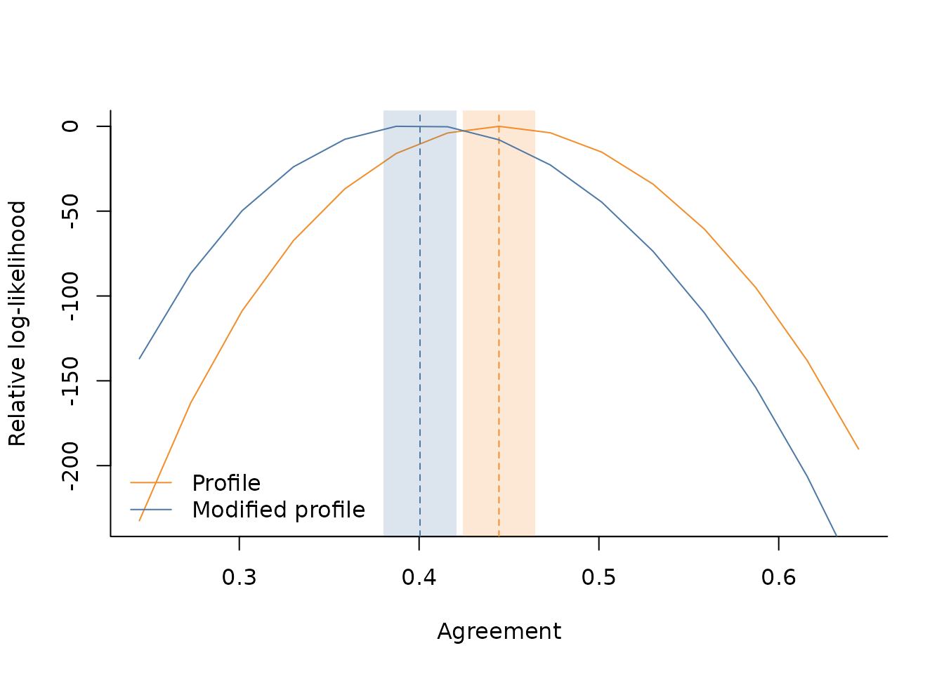
#> [1] 0.3802357 0.4207772

For convenience, we provide a utility function to visualise the relative log-likelihood profiles of the two methods as well as the inference results

# compute log-likelihood over a grid
range_ll <- get_range_ll(fit_modified)

# utility plot function for relative log-likelihood
plot_rll(
  D=range_ll,
  M_EST = fit_modified$modified$agreement,
  P_EST = fit_profile$profile$agreement,
  M_SE = ci_modified$agreement_se,
  P_SE = ci_profile$agreement_se,
  CONFIDENCE=.95
)