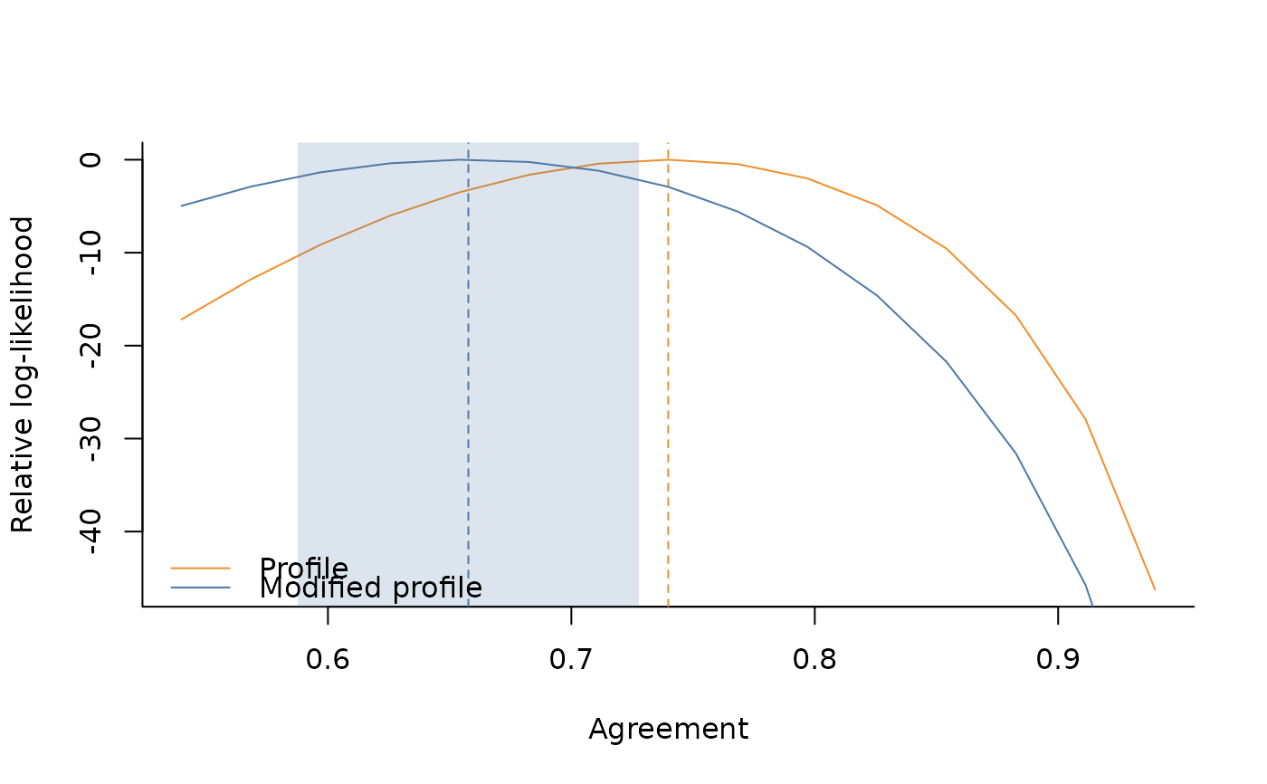
Plot relative log-likelihood

Plot relative log-likelihood

Usage

plot_rll(
  D,
  M_EST = NULL,
  P_EST = NULL,
  M_SE = NULL,
  P_SE = NULL,
  CONFIDENCE = 0.95
)

Arguments

D

output from get_range_ll

M_EST

agreement estimate from modified profile likelihood

P_EST

agreement estimate from profile likelihood

M_SE

standard error for agreement estimate from modified profile likelihood

P_SE

standard error for agreement estimate from profile likelihood

CONFIDENCE

Confidence level to construct confidence intervals

Examples

set.seed(321)

# setting dimension
items <- 50
budget_per_item <- 5
n_obs <- items * budget_per_item
workers <- 50

# item-specific intercepts to generate the data
alphas <- runif(items, -2, 2)

# true agreement (between 0 and 1)
agr <- .6

# generate continuous rating in (0,1)
dt_oneway <- sim_data(
  J = items,
  B = budget_per_item,
  AGREEMENT = agr,
  ALPHA = alphas,
  DATA_TYPE = "continuous",
  SEED = 123
)

# estimation via oneway specification
fit <- agreement(
  RATINGS = dt_oneway$rating,
  ITEM_INDS = dt_oneway$id_item,
  WORKER_INDS = dt_oneway$id_worker,
  METHOD = "modified",
  NUISANCE = c("items"),
  VERBOSE = TRUE
)
#> 
#> DATA
#>  - Detected 50 items and 49 workers.
#>  - Detected continuous data on the (0,1) range.
#>  - Average number of observed ratings per item is 5.
#>  - Average number of observed ratings per worker is 5.1.
#> 
#> MODEL PARAMETERS
#>  - Constant effects: workers
#>  - Nuisance effects: items
#> Non-adjusted agreement: 0.739811
#> Adjusted agreement: 0.657685
#> Done!
# get standard error and confidence interval
ci <- get_ci(fit)
ci
#> $agreement_est
#> [1] 0.6576846
#> 
#> $agreement_se
#> [1] 0.03584845
#> 
#> $agreement_ci
#> [1] 0.5874229 0.7279463
#> 

# compute log-likelihood over a grid
range_ll <- get_range_ll(fit)

# utility plot function for relative log-likelihood
plot_rll(
  D = range_ll,
  M_EST = fit$modified$agreement,
  P_EST = fit$profile$agreement,
  M_SE = ci$agreement_se,
  CONFIDENCE=.95
)