Solutions Lab 4 practice

Practice 1

For importing, use the read_xlsx()function and specify the sheet argument.

library(readxl)
library(tidyverse)

# declare where you are in your project folder
i_am("practice1.R")

# construct the path to your data
path <- here("data", "ecommerce.xlsx")

# read the two sheets by specifying the "sheet" argument
purchases <- read_xlsx(path = path, sheet = "purchases_history")
products  <- read_xlsx(path = path, sheet = "products")

Exercise 1

library(janitor)

purchases <- purchases |> clean_names()
products <- products |> clean_names()

To compute the total number of sales by product we can use the group_by() + summarise() combo.

purchases |> 
    group_by(product) |> 
    summarise(
        number_of_sales = n()
    )

# A tibble: 7 × 2
  product      number_of_sales
  <chr>                  <int>
1 e-reader                  96
2 earphones                115
3 laptop_1                  48
4 laptop_2                  46
5 smartphone_1              49
6 smartphone_2              52
7 tablet                    94

There is even a faster way to count how many times the values of a given variable appear in the dataset. Literally, you can pipe the count() function

purchases |> 
    count(product)

# A tibble: 7 × 2
  product          n
  <chr>        <int>
1 e-reader        96
2 earphones      115
3 laptop_1        48
4 laptop_2        46
5 smartphone_1    49
6 smartphone_2    52
7 tablet          94

Exercise 2

To compute the total amount of money spent on each product we first join the two datasets,

purchases |> 
    left_join(products, by = "product") 

# A tibble: 500 × 3
   customer_id                          product      price_euro
   <chr>                                <chr>             <dbl>
 1 1609fdd7-29c6-4678-84af-30684d709f0b earphones          90.0
 2 1064a4dc-df76-4aba-8b74-953a4c66fa16 smartphone_1      500. 
 3 155e9331-3434-415f-9d66-67736534d80b e-reader          200. 
 4 105696b8-7c38-4fe5-92f5-3c6fb1268f48 laptop_2          900. 
 5 12175814-556e-4e1a-af05-0c38c13e98a0 laptop_1         2140. 
 6 80fb4c6d-d5f8-42ed-b3c7-8a10596dd382 tablet            520. 
 7 348651a5-8a5a-4311-b999-4dfba846a413 e-reader          200. 
 8 cea15e94-869f-417a-9ad4-a70aefc74f34 laptop_2          900. 
 9 8b0a0720-0487-44d2-9aae-32dfec5c4b5c e-reader          200. 
10 578ffa9d-ec4c-4a54-8a32-6f15ac4deb53 e-reader          200. 
# ℹ 490 more rows

and then comput the totals,

purchases |> 
    left_join(products, by = "product") |> 
    group_by(product) |> 
    summarise(
        total = sum(price_euro),
        total_thousands = sum(price_euro)/1000
        )

# A tibble: 7 × 3
  product        total total_thousands
  <chr>          <dbl>           <dbl>
1 e-reader      19199.            19.2
2 earphones     10349.            10.3
3 laptop_1     102720.           103. 
4 laptop_2      41400.            41.4
5 smartphone_1  24500.            24.5
6 smartphone_2  15599.            15.6
7 tablet        48879.            48.9

Equivalently, we can also first count how many items have been sold by product type, as in the previous exercise, and then join the resulting table with the price listings

purchases |> 
    count(product) |> 
    left_join(products)

# A tibble: 7 × 3
  product          n price_euro
  <chr>        <int>      <dbl>
1 e-reader        96      200. 
2 earphones      115       90.0
3 laptop_1        48     2140. 
4 laptop_2        46      900. 
5 smartphone_1    49      500. 
6 smartphone_2    52      300. 
7 tablet          94      520. 

Once here, we need to compute total by product by multiplying their prices and quantities sold

purchases |> 
    count(product) |> 
    left_join(products) |> 
    mutate(
        total_thousands = price_euro * n /1000
    )

# A tibble: 7 × 4
  product          n price_euro total_thousands
  <chr>        <int>      <dbl>           <dbl>
1 e-reader        96      200.             19.2
2 earphones      115       90.0            10.3
3 laptop_1        48     2140.            103. 
4 laptop_2        46      900.             41.4
5 smartphone_1    49      500.             24.5
6 smartphone_2    52      300.             15.6
7 tablet          94      520.             48.9

Practice 2

Exercise 1

library(readxl)
library(tidyverse)

# declare where you are in your project folder
i_am("practice2.R")

# construct the path to your data
path <- here("data", "avocados.xlsx")

avocados <- read_xlsx(path = path)

We need to use pivot_longer() to reshape the data:

new_avo <- avocados |> 
  pivot_longer(
    cols = c(conventional, organic), 
    names_to = "type", 
    values_to = "avg_price"
    ) 
new_avo

# A tibble: 338 × 3
   date                type         avg_price
   <dttm>              <chr>            <dbl>
 1 2015-01-04 00:00:00 conventional     1.01 
 2 2015-01-04 00:00:00 organic          1.59 
 3 2015-01-11 00:00:00 conventional     1.11 
 4 2015-01-11 00:00:00 organic          1.63 
 5 2015-01-18 00:00:00 conventional     1.13 
 6 2015-01-18 00:00:00 organic          1.65 
 7 2015-01-25 00:00:00 conventional     1.12 
 8 2015-01-25 00:00:00 organic          1.68 
 9 2015-02-01 00:00:00 conventional     0.962
10 2015-02-01 00:00:00 organic          1.53 
# ℹ 328 more rows

Once reshaped, we can plot the price trajectories over time:

new_avo |> 
  ggplot(aes(x=date, y=avg_price, col=type))+
  geom_line()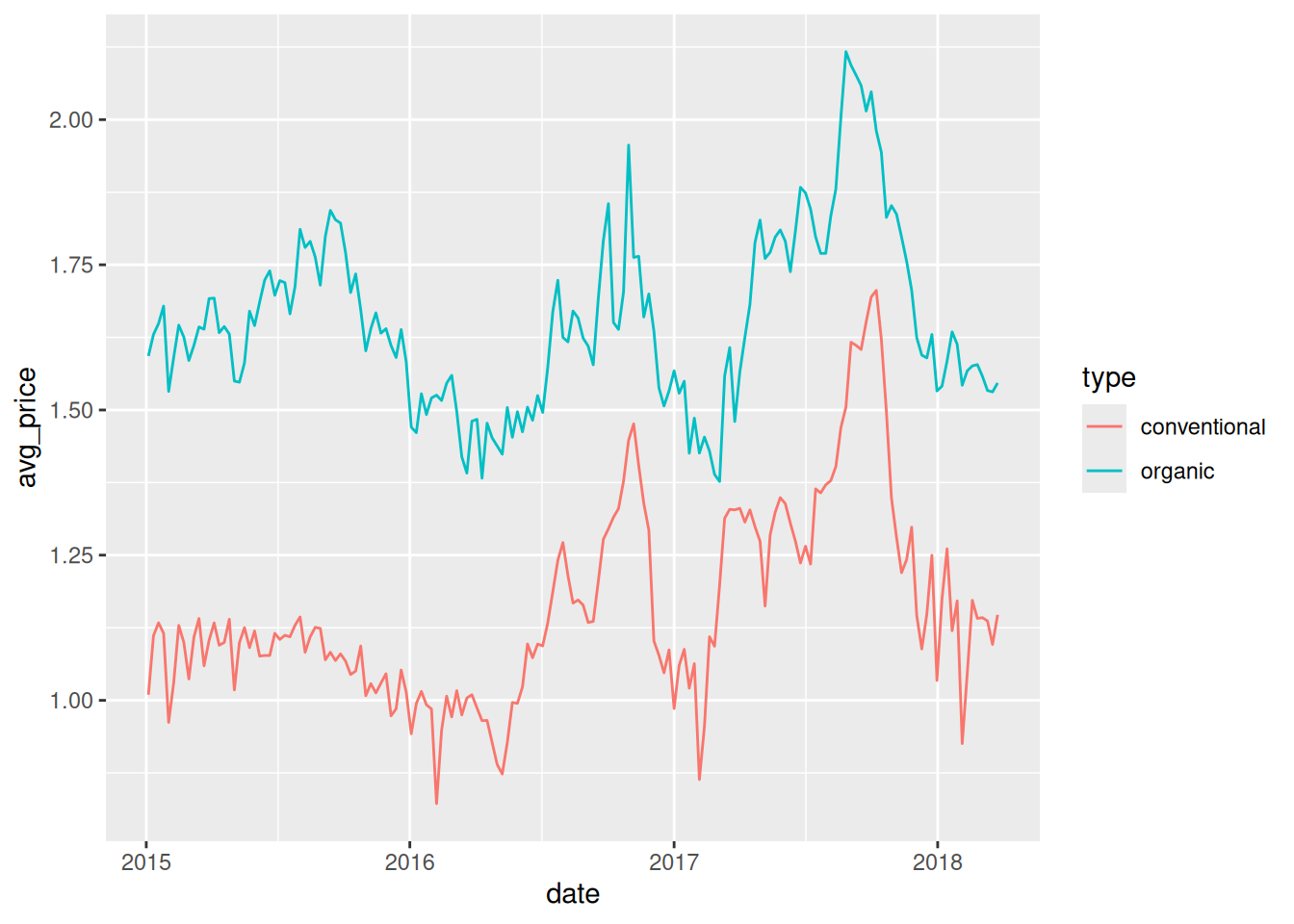

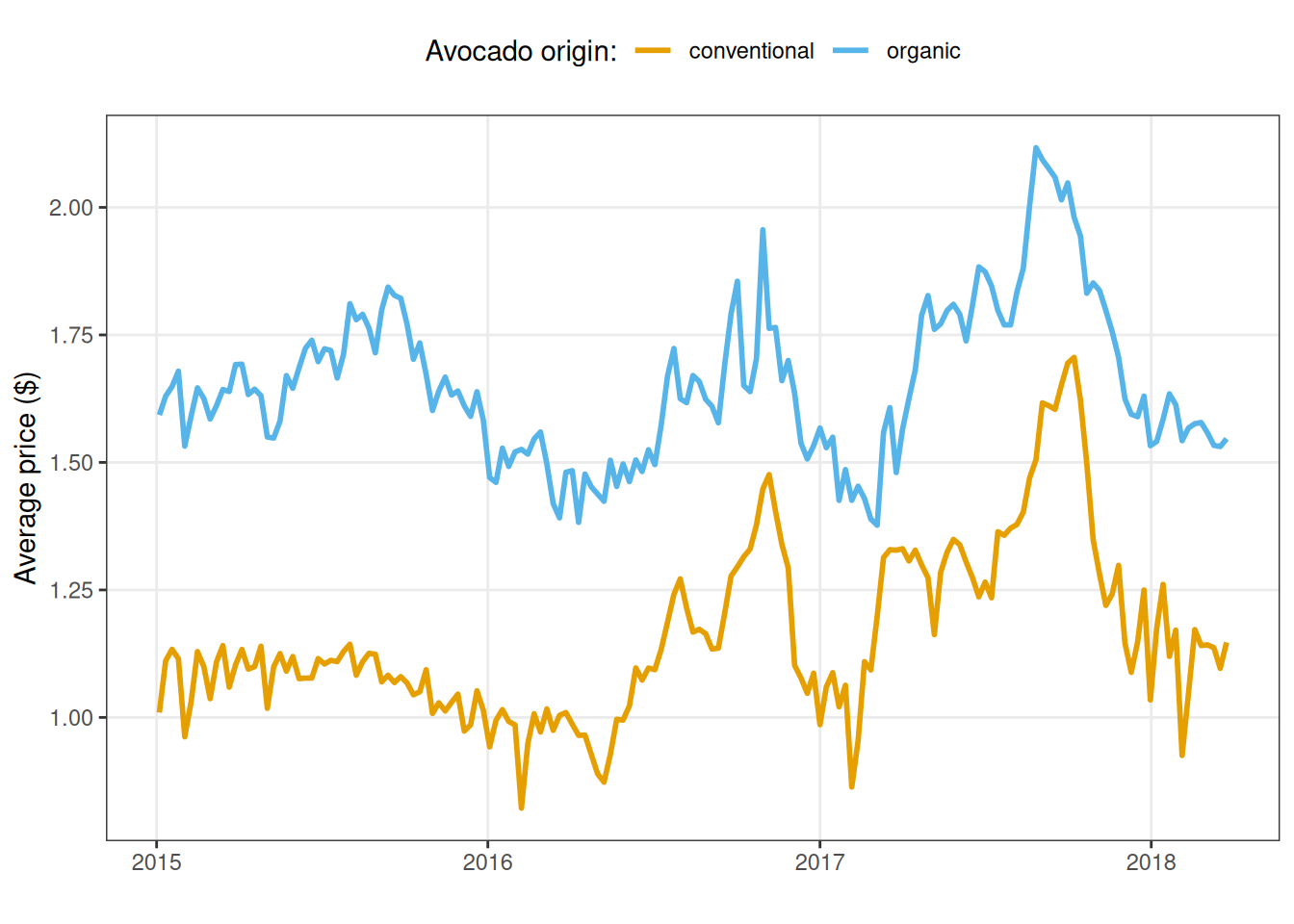
As always, we can customise the plots as we prefer:

library(ggokabeito)
new_avo |> 
  ggplot(aes(x=date, y=avg_price, col=type))+
  geom_line(linewidth=1) +
  labs(x="", y= "Average price ($)", color="Avocado origin:")+
  theme_bw() +
  theme(
    legend.position = "top", 
    panel.grid.minor = element_blank()
    )+
  scale_color_okabe_ito()